How To Highlight Entire Row Based On Cell Value In Excel
How To Highlight Entire Row Based On Cell Value In Excel - There are a lot of affordable templates out there, but it can be easy to feel like a lot of the best cost a amount of money, require best special design template. Making the best template format choice is way to your template success. And if at this time you are looking for information and ideas regarding the How To Highlight Entire Row Based On Cell Value In Excel then, you are in the perfect place. Get this How To Highlight Entire Row Based On Cell Value In Excel for free here. We hope this post How To Highlight Entire Row Based On Cell Value In Excel inspired you and help you what you are looking for.
“`html
Highlighting entire rows in Excel based on a cell value is a powerful technique for visually emphasizing important data and improving the readability of your spreadsheets. It allows you to quickly identify rows that meet specific criteria without having to manually scan each cell.
Using Conditional Formatting
The most common and efficient way to highlight entire rows based on a cell value is through Excel’s Conditional Formatting feature. Here’s a step-by-step guide:
1. Select the Data Range
First, you need to select the range of cells you want to apply the formatting to. This is crucial because Excel will use the selected range to determine which rows to highlight. You’ll want to select the entire data set, including all the columns you want highlighted when the condition is met. For example, if your data starts in cell A1 and extends to cell G100, you would select the range A1:G100.
2. Access Conditional Formatting
Navigate to the Home tab on the Excel ribbon. In the Styles group, you’ll find the Conditional Formatting button. Click it to open the Conditional Formatting menu.
3. Create a New Rule
From the Conditional Formatting menu, select New Rule…. This will open the “New Formatting Rule” dialog box.
4. Choose a Rule Type
In the “New Formatting Rule” dialog box, you’ll see several rule types. Choose the option that says: “Use a formula to determine which cells to format”.
5. Enter the Formula
This is the heart of the process. You’ll now enter a formula that Excel will use to evaluate each row in your selected range. The formula must return either TRUE or FALSE. If the formula evaluates to TRUE for a particular row, that row will be formatted. The key is to understand how Excel iterates through the selected range.first cell in that row as the reference point.Here’s the general structure of the formula:
=$ColumnLetter$RowNumber= "YourCriteria"
Let’s break this down:
=: This signifies that you’re starting a formula.$ColumnLetter: This is the column letter of the cell you want to check. The$(dollar sign) is very important here. It makes the column reference absolute. This means that when Excel applies the formula to other rows, it will always refer to the specified column.$RowNumber: This is the starting row number of your selected range. For example, if you selected A1:G100, the row number would be 1. Using a dollar sign here would prevent the conditional formatting from working correctly. We want the row number to be relative so that excel can iterate over each row.=: This is the comparison operator. You can use other operators like<(less than),>(greater than),<=(less than or equal to),>=(greater than or equal to), or<>(not equal to)."YourCriteria": This is the value you’re comparing the cell to. It can be text (enclosed in double quotes), a number, a date, or even a reference to another cell (e.g.,=$A1=$H1).
Examples:
- Highlight rows where the value in column A is “Completed”:
=$A1="Completed" - Highlight rows where the value in column B is greater than 100:
=$B1>100 - Highlight rows where the value in column C is equal to the value in cell H1:
=$C1=$H$1(Note the$signs around H1 to make it an absolute reference, so it doesn’t change when the formula is applied to other rows.) - Highlight rows where the value in column D is a date before 1/1/2024:
=$D1<DATE(2024,1,1) - Highlight rows where column E is blank:
=ISBLANK($E1) - Highlight rows where column F contains the text “Error”:
=ISNUMBER(SEARCH("Error",$F1))
Enter your formula in the formula box provided in the “New Formatting Rule” dialog box.
6. Choose the Formatting
Click the Format… button. This opens the “Format Cells” dialog box. Here, you can specify the formatting you want to apply to the highlighted rows. You can change the font (style, color, size), the fill color (background color), the border, and other formatting options.
For example, you might choose to fill the rows with a light green color, or make the text bold.
7. Apply the Rule
Click OK in both the “Format Cells” and “New Formatting Rule” dialog boxes. Excel will now apply the conditional formatting to your selected range.
8. Manage Conditional Formatting Rules (Optional)
To modify or delete a conditional formatting rule, go back to Conditional Formatting on the Home tab and select Manage Rules…. In the “Conditional Formatting Rules Manager” dialog box, you can see all the rules applied to the current sheet, edit them, delete them, or change their order of precedence.
Important Considerations
* **Absolute vs. Relative References:** The use of $ (dollar signs) is critical. Using $A1 makes the column absolute but the row relative. This allows Excel to correctly apply the formula to each row. Using A1 with no dollar signs makes both the column and row relative which will cause the conditional formatting to not work as expected. Using $A$1 makes both the column and row absolute, causing all rows to be highlighted (or none) depending on the value in cell A1. * **Formula Complexity:** You can create very complex formulas using Excel’s built-in functions (AND, OR, NOT, ISBLANK, SEARCH, etc.). This allows you to create rules based on multiple conditions. For example, you could highlight rows where column A is “Completed” AND column B is greater than 100. * **Rule Order:** If you have multiple conditional formatting rules that overlap, the order in which they are applied matters. You can change the order in the “Conditional Formatting Rules Manager”. The rule at the top of the list takes precedence. * **Performance:** Applying conditional formatting to very large datasets can sometimes impact performance. If you notice slowdowns, try to simplify your formulas or reduce the size of the data range you’re applying the formatting to. * **Clear Formatting:** To remove conditional formatting, select the range, go to Conditional Formatting, and choose Clear Rules. You can clear rules from the selected cells or from the entire sheet. * **Copying Formatting:** You can use the “Format Painter” (on the Home tab) to copy conditional formatting from one range to another. This is a quick way to apply the same rules to multiple areas of your spreadsheet. * **Using Named Ranges:** Instead of directly referencing cells like $A1, you can use named ranges. This makes your formulas more readable and easier to maintain. For example, if you named column A “Status”, your formula could be =Status1="Completed".
Example: Highlighting Overdue Tasks
Let’s say you have a task list with columns for “Task Name” (A), “Due Date” (B), and “Status” (C). You want to highlight rows where the due date is in the past AND the status is not “Completed”.
- Select your data range (e.g., A2:C100).
- Go to Conditional Formatting -> New Rule…
- Choose “Use a formula to determine which cells to format”.
- Enter the following formula:
=AND($B2<TODAY(),$C2<>"Completed") - Click “Format…” and choose a highlight color (e.g., red).
- Click OK to apply the rule.
This formula uses the AND function to combine two conditions: $B2<TODAY() (the due date is before today) and $C2<>"Completed" (the status is not equal to “Completed”). Only rows that meet both conditions will be highlighted.
By mastering conditional formatting, you can create dynamic and visually informative spreadsheets that help you analyze data and make better decisions.
“`
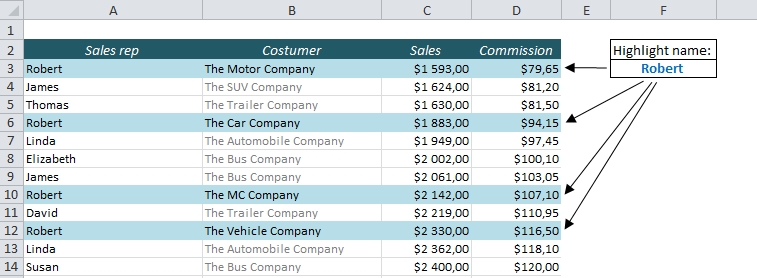 757×278 highlight entire row excel based cell easy excelcom from easy-excel.com
 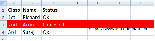 520×138 highlight entire row excel based cell vba from www.encodedna.com
  716×444 highlight rows based cell excel conditional formatting from trumpexcel.com
 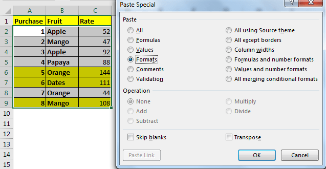 474×245 highlight row base cell excel from www.exceltip.com
  474×372 highlight row based cell number conditional formula from yodalearning.com
  1200×1142 highlight entire rows based cell excel hubpages from discover.hubpages.com
  1099×462 highlight rows based cell excel geeksforgeeks from www.geeksforgeeks.org
 How To Highlight Entire Row Based On Cell Value In Excel was posted in September 8, 2025 at 11:43 am. If you wanna have it as yours, please click the Pictures and you will go to click right mouse then Save Image As and Click Save and download the How To Highlight Entire Row Based On Cell Value In Excel Picture.. Don’t forget to share this picture with others via Facebook, Twitter, Pinterest or other social medias! we do hope you'll get inspired by ExcelKayra... Thanks again! If you have any DMCA issues on this post, please contact us!