How To Use Iferror Function In Excel With Examples
How To Use Iferror Function In Excel With Examples - There are a lot of affordable templates out there, but it can be easy to feel like a lot of the best cost a amount of money, require best special design template. Making the best template format choice is way to your template success. And if at this time you are looking for information and ideas regarding the How To Use Iferror Function In Excel With Examples then, you are in the perfect place. Get this How To Use Iferror Function In Excel With Examples for free here. We hope this post How To Use Iferror Function In Excel With Examples inspired you and help you what you are looking for.
“`html
Understanding and Using the IFERROR Function in Excel
The IFERROR function in Excel is a powerful tool for handling errors gracefully within your formulas. Instead of displaying unsightly error messages like #DIV/0!, #N/A, #NAME?, #NULL!, #NUM!, #REF!, or #VALUE!, IFERROR allows you to specify an alternative value to be displayed when an error occurs. This can significantly improve the readability and professionalism of your spreadsheets.
Syntax of the IFERROR Function
The syntax of the IFERROR function is simple:
IFERROR(value, value_if_error)Where:
value: This is the expression, formula, or value that you want to evaluate. It’s the argument that Excel will attempt to calculate.value_if_error: This is the value that will be returned if thevalueargument results in an error. This can be a specific value, another formula, or even an empty string (“”).
How IFERROR Works
The IFERROR function checks the first argument (value). If the value argument evaluates without an error, IFERROR returns the result of the value argument. However, if the value argument results in any of the Excel error types mentioned earlier, IFERROR returns the value_if_error argument.
Practical Examples of Using IFERROR
Here are several examples illustrating how to use the IFERROR function in various scenarios:
1. Handling Division by Zero Errors
One of the most common uses of IFERROR is to prevent division by zero errors (#DIV/0!). Imagine you have a spreadsheet calculating percentages, and sometimes the denominator is zero.
Suppose cell A1 contains the numerator (e.g., 10) and cell B1 contains the denominator (e.g., 0). Without IFERROR, the formula =A1/B1 would result in #DIV/0!. To handle this, use:
=IFERROR(A1/B1, 0)This formula will now return 0 when B1 is zero (or any value that causes a division by zero error). You could also return a text string indicating the error:
=IFERROR(A1/B1, "Denominator is zero")This would display “Denominator is zero” in the cell if B1 is zero.
2. Preventing #N/A Errors with VLOOKUP
The VLOOKUP function returns #N/A when it cannot find the lookup value in the specified table. IFERROR can make your VLOOKUP formulas more robust.
Let’s say you’re using VLOOKUP to find a product price from a table. The formula might look like this:
=VLOOKUP(D1, A1:B10, 2, FALSE)Where:
D1: The product name you’re looking for.A1:B10: The range containing the product names (column A) and prices (column B).2: The column number (price is in the second column).FALSE: Specifies an exact match.
If the product in D1 is not found in the range A1:B10, the formula will return #N/A. To handle this, you can use:
=IFERROR(VLOOKUP(D1, A1:B10, 2, FALSE), "Product not found")This will display “Product not found” if the product name isn’t found in the table. Alternatively, you could return an empty string:
=IFERROR(VLOOKUP(D1, A1:B10, 2, FALSE), "")This would leave the cell blank if the product isn’t found.
3. Handling Errors in Complex Calculations
IFERROR is particularly useful when dealing with complex formulas that involve multiple calculations, where errors might arise from various sources.
For example, consider a formula that calculates the average of a range of cells, but you want to exclude any cells that contain errors:
=IFERROR(AVERAGE(A1:A10), "Error in data")However, this only handles an error returned by the AVERAGE function itself. If any individual cell in the range A1:A10 *already* contains an error, the AVERAGE function will return an error. You might want to first handle those errors:
=AVERAGE(IFERROR(A1:A10,0))This cleverly replaces any errors within the A1:A10 range with 0 before the AVERAGE is calculated. Note this is an array formula and needs to be entered with CTRL+SHIFT+ENTER.
You can combine the above:
=IFERROR(AVERAGE(IFERROR(A1:A10,0)),"No Valid Data")This handles both errors in the data and cases where all cells contain errors, resulting in the AVERAGE function returning an error.
4. Returning Different Values Based on the Error
While IFERROR doesn’t directly identify *which* error occurred, you can nest IFERROR functions to handle specific error types differently, although this can quickly become complex.
For example, you might want to return a different message for #DIV/0! errors compared to #N/A errors. While IFERROR doesn’t directly distinguish between error types, you can utilize helper columns or more complex formulas to identify the specific error and provide tailored responses.
5. Using IFERROR with INDEX and MATCH
The INDEX and MATCH functions are often used together to perform advanced lookups. Like VLOOKUP, MATCH can return #N/A if a match isn’t found.
Consider a formula that uses INDEX and MATCH to find the name of a customer based on their ID:
=INDEX(A1:A10, MATCH(E1, B1:B10, 0))Where:
A1:A10: The range containing customer names.E1: The customer ID you’re looking for.B1:B10: The range containing customer IDs.0: Specifies an exact match.
If the customer ID in E1 isn’t found in the range B1:B10, MATCH returns #N/A, causing INDEX to also return #N/A. To handle this, use:
=IFERROR(INDEX(A1:A10, MATCH(E1, B1:B10, 0)), "Customer ID not found")This will display “Customer ID not found” if the ID isn’t found.
Best Practices When Using IFERROR
- Use it selectively: Avoid wrapping every formula in
IFERROR. Only use it where you anticipate potential errors and want to handle them gracefully. OverusingIFERRORcan mask underlying problems with your data or formulas. - Choose appropriate error values: Consider what value makes the most sense to return when an error occurs. An empty string, zero, or a descriptive text message are common choices.
- Test your formulas: Always test your formulas with different inputs, including edge cases and invalid data, to ensure that
IFERRORis working as expected. - Consider alternative solutions: In some cases, there might be a better way to prevent errors in the first place. For example, validating data input or cleaning your data might eliminate the need for
IFERRORin some situations.
Conclusion
The IFERROR function is a valuable tool for creating more robust and user-friendly Excel spreadsheets. By handling errors gracefully, you can prevent unsightly error messages, improve the readability of your data, and ensure that your calculations produce meaningful results. By understanding its syntax and applying it strategically, you can leverage IFERROR to enhance the overall quality and professionalism of your Excel work.
“`
 1281×662 excel iferror function excelfind from excelfind.com
  622×182 excel iferror function excel vba from www.exceldome.com
 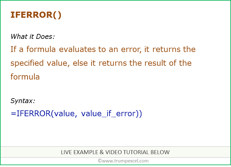 752×546 excel iferror function formula examples video from trumpexcel.com
 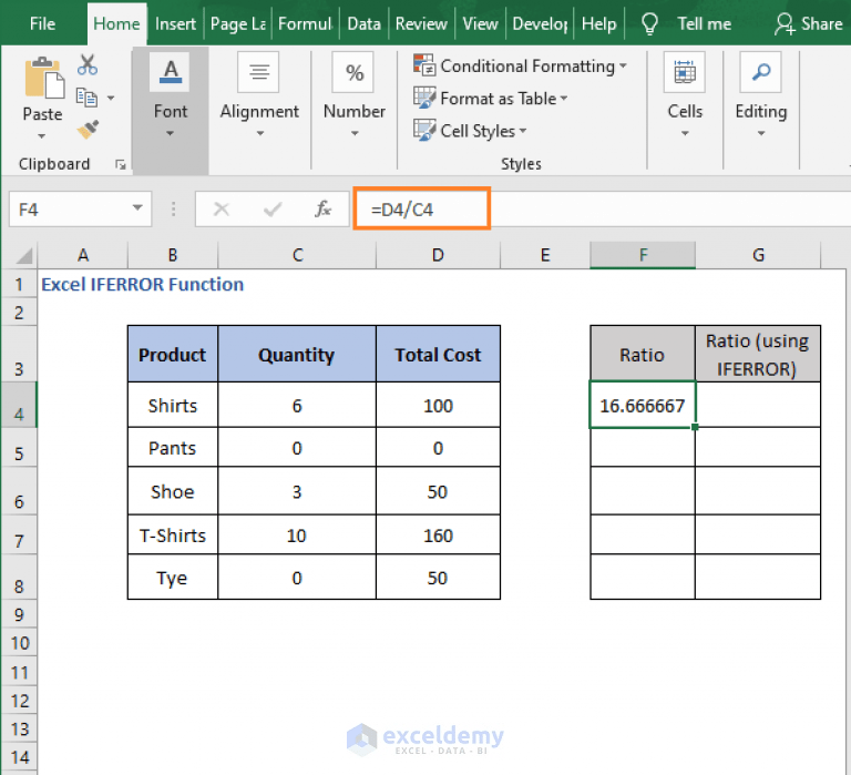 768×699 iferror function excel examples exceldemy from www.exceldemy.com
  700×400 excel iferror function exceljet from exceljet.net
  876×717 iferror function excel remove excel error excel unlocked from excelunlocked.com
  1024×478 iferror function excel examples geeksforgeeks from www.geeksforgeeks.org
  604×267 iferror function excel step step tutorial from www.excel-easy.com
  768×511 iferror function excel from www.exceltip.com
  469×179 iferror excel formula examples ablebitscom from www.ablebits.com
 How To Use Iferror Function In Excel With Examples was posted in January 4, 2026 at 5:51 pm. If you wanna have it as yours, please click the Pictures and you will go to click right mouse then Save Image As and Click Save and download the How To Use Iferror Function In Excel With Examples Picture.. Don’t forget to share this picture with others via Facebook, Twitter, Pinterest or other social medias! we do hope you'll get inspired by ExcelKayra... Thanks again! If you have any DMCA issues on this post, please contact us!