How To Use Sumifs Function In Excel With Examples
How To Use Sumifs Function In Excel With Examples - There are a lot of affordable templates out there, but it can be easy to feel like a lot of the best cost a amount of money, require best special design template. Making the best template format choice is way to your template success. And if at this time you are looking for information and ideas regarding the How To Use Sumifs Function In Excel With Examples then, you are in the perfect place. Get this How To Use Sumifs Function In Excel With Examples for free here. We hope this post How To Use Sumifs Function In Excel With Examples inspired you and help you what you are looking for.
“`html
Understanding and Using the SUMIFS Function in Excel
The SUMIFS function in Excel is a powerful tool for calculating the sum of values in a range based on multiple criteria. It allows you to add up numbers only when specific conditions are met in corresponding ranges. This is incredibly useful for analyzing data, creating reports, and gaining deeper insights from your spreadsheets. Unlike the SUMIF function, which only accepts a single condition, SUMIFS allows for multiple conditions, making it significantly more versatile.
Syntax of SUMIFS
The syntax of the SUMIFS function is as follows:
SUMIFS(sum_range, criteria_range1, criteria1, [criteria_range2, criteria2], ...) Let’s break down each argument:
- sum_range: This is the range of cells containing the values you want to sum. Only the cells within this range that meet all the specified criteria will be added.
- criteria_range1: This is the range of cells where you want to apply the first criterion. It should have the same dimensions as the `sum_range` if you want to apply the criteria directly to the values being summed.
- criteria1: This is the first criterion that will be used to filter the `sum_range`. It can be a number, a text string, a date, a logical expression, or a reference to another cell containing the criteria.
- [criteria_range2, criteria2], …: These are optional arguments. You can specify up to 127 pairs of criteria ranges and criteria. Each pair represents an additional condition that must be met for a value in the `sum_range` to be included in the sum.
Key Considerations When Using SUMIFS
- Range Sizes: All `criteria_range` arguments must have the same number of rows and columns as the `sum_range`. Excel will return a #VALUE! error if the ranges are not the same size and shape.
- Multiple Criteria: The SUMIFS function only adds values if all the specified criteria are met. It’s an AND condition – not an OR condition.
- Wildcards: You can use wildcard characters like the asterisk (*) to represent any sequence of characters and the question mark (?) to represent any single character within the criteria. This is useful for partial matches.
- Logical Operators: You can use logical operators (>, <, >=, <=, <>) within your criteria to create more complex conditions. These operators must be enclosed in double quotes and concatenated with the cell reference or value using the ampersand (&) symbol.
- Blank Cells: Blank cells in a criteria range will be treated as zero values in numerical criteria, and as empty strings in text criteria.
- Case-Insensitivity: The SUMIFS function is generally case-insensitive when dealing with text criteria.
Examples of SUMIFS in Action
Let’s illustrate how to use the SUMIFS function with practical examples.
Example 1: Summing Sales by Region and Product
Suppose you have a table of sales data with columns for Region, Product, and Sales Amount. You want to calculate the total sales amount for a specific region and a specific product.
Your data might look like this:
| Region | Product | Sales Amount |
|---|---|---|
| North | Apples | 100 |
| South | Bananas | 150 |
| North | Bananas | 200 |
| East | Apples | 120 |
| North | Apples | 80 |
| South | Oranges | 180 |
Assume this data is in cells A2:C7. To calculate the total sales for “North” region and “Apples” product, you would use the following formula:
=SUMIFS(C2:C7, A2:A7, "North", B2:B7, "Apples") Explanation:
- `C2:C7` is the `sum_range` (Sales Amount).
- `A2:A7` is the `criteria_range1` (Region).
- `”North”` is the `criteria1` (Region must be “North”).
- `B2:B7` is the `criteria_range2` (Product).
- `”Apples”` is the `criteria2` (Product must be “Apples”).
The result of this formula would be 180 (100 + 80).
Example 2: Summing Sales Greater Than a Certain Value
Let’s say you want to sum sales amounts only for orders that exceeded $100. Continuing with the same data structure, you can use a logical operator in your criteria.
=SUMIFS(C2:C7, C2:C7, ">100") Explanation:
- `C2:C7` is the `sum_range` (Sales Amount).
- `C2:C7` is also the `criteria_range1` (Sales Amount). In this case we are applying the condition directly on the values we are summing.
- `”>100″` is the `criteria1` (Sales Amount must be greater than 100).
The result of this formula would be 650 (150 + 200 + 120 + 180).
Example 3: Summing Sales Based on Date Ranges
Imagine you have a Date column along with Region, Product and Sales Amount. You want to sum sales for a specific date range.
Expanded Data Example:
| Date | Region | Product | Sales Amount |
|---|---|---|---|
| 1/1/2024 | North | Apples | 100 |
| 1/5/2024 | South | Bananas | 150 |
| 1/10/2024 | North | Bananas | 200 |
| 1/15/2024 | East | Apples | 120 |
| 1/20/2024 | North | Apples | 80 |
| 1/25/2024 | South | Oranges | 180 |
Assume the data is in cells A2:D7. To sum sales between January 5th, 2024 and January 20th, 2024 (inclusive), you would use:
=SUMIFS(D2:D7, A2:A7, ">=1/5/2024", A2:A7, "<=1/20/2024") Explanation:
- `D2:D7` is the `sum_range` (Sales Amount).
- `A2:A7` is the `criteria_range1` (Date).
- `">=1/5/2024"` is the `criteria1` (Date must be greater than or equal to January 5th, 2024).
- `A2:A7` is the `criteria_range2` (Date - again).
- `"<=1/20/2024"` is the `criteria2` (Date must be less than or equal to January 20th, 2024).
The result would be 550 (150 + 200 + 120 + 80).
Example 4: Using Cell References for Criteria
Instead of hardcoding criteria directly into the formula, you can use cell references. This makes your formulas more dynamic and easier to update.
Let's say cell F1 contains "North" and cell F2 contains "Apples". You can rewrite Example 1 as:
=SUMIFS(C2:C7, A2:A7, F1, B2:B7, F2) Now, if you change the values in F1 and F2, the SUMIFS formula will automatically recalculate based on the new criteria.
Example 5: Using Wildcards
If you want to sum sales for all products that start with "A", you can use the wildcard character "*":
=SUMIFS(C2:C7, B2:B7, "A*") This would sum sales for "Apples" in our original data (resulting in 100 + 80 + 120 = 300).
Example 6: Combining Logical Operators and Cell References
Suppose cell F3 contains the number 120. You want to sum sales amounts that are greater than the value in cell F3.
=SUMIFS(C2:C7, C2:C7, ">"&F3) Explanation:
- `C2:C7` is the `sum_range` (Sales Amount).
- `C2:C7` is the `criteria_range1` (Sales Amount).
- `">"&F3` concatenates the ">" operator with the value in cell F3 (which is 120), resulting in the criterion ">120".
The result would be 150 + 200 + 180 = 530.
Troubleshooting SUMIFS Errors
- #VALUE! Error: This usually indicates that the `sum_range` and `criteria_range` arguments do not have the same dimensions. Ensure they have the same number of rows and columns.
- Incorrect Results: Double-check your criteria to ensure they accurately reflect the conditions you want to apply. Make sure you're using the correct logical operators and that cell references are pointing to the correct cells. Also, verify that your date formats are consistent (Excel can misinterpret dates if the format is incorrect).
- No Results (Zero Sum): If the result is zero, it means no values in the `sum_range` met all the specified criteria. Carefully review your criteria and data to identify any discrepancies.
Conclusion
The SUMIFS function is a powerful and flexible tool for conditional summing in Excel. By mastering its syntax and understanding how to use criteria, logical operators, and wildcards, you can effectively analyze your data and gain valuable insights. Practice with different scenarios and data sets to become proficient in using SUMIFS and unlock its full potential.
```
 752×551 excel sumifs function examples video from trumpexcel.com
 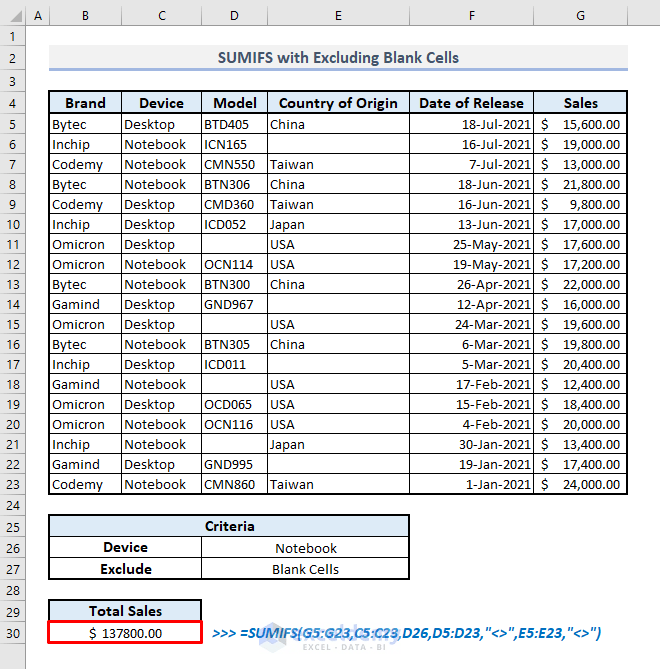 660×669 sumifs function excel handy examples exceldemy from www.exceldemy.com
  1202×684 sumifs function excelnotes from excelnotes.com
 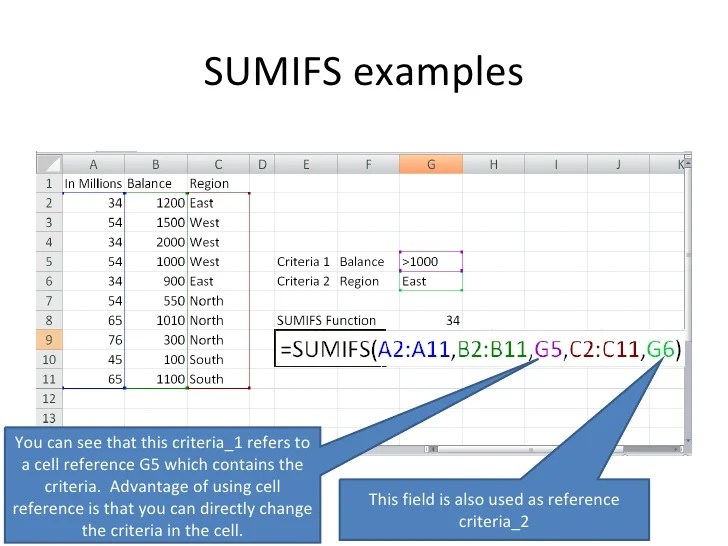 728×546 excel sumifs function from www.slideshare.net
  644×390 sumifs function excel from www.exceltip.com
  1080×423 sumifs function excel formula examples from spreadsheetweb.com
  637×258 excel sumif sumifs explained from www.exceltrick.com
 How To Use Sumifs Function In Excel With Examples was posted in November 23, 2025 at 4:45 pm. If you wanna have it as yours, please click the Pictures and you will go to click right mouse then Save Image As and Click Save and download the How To Use Sumifs Function In Excel With Examples Picture.. Don’t forget to share this picture with others via Facebook, Twitter, Pinterest or other social medias! we do hope you'll get inspired by ExcelKayra... Thanks again! If you have any DMCA issues on this post, please contact us!