Home » Excel Templates » How To Use The Iferror Function To Handle Errors In Excel

How To Use The Iferror Function To Handle Errors In Excel

Friday, August 22nd 2025. | Excel Templates

How To Use The Iferror Function To Handle Errors In Excel - There are a lot of affordable templates out there, but it can be easy to feel like a lot of the best cost a amount of money, require best special design template. Making the best template format choice is way to your template success. And if at this time you are looking for information and ideas regarding the How To Use The Iferror Function To Handle Errors In Excel then, you are in the perfect place. Get this How To Use The Iferror Function To Handle Errors In Excel for free here. We hope this post How To Use The Iferror Function To Handle Errors In Excel inspired you and help you what you are looking for.

excel iferror function formula examples video

“`html

Handling Errors Gracefully in Excel with IFERROR

Excel is a powerful tool for data analysis and manipulation. However, formulas, especially complex ones, can sometimes produce errors. These errors, such as #DIV/0!, #VALUE!, #REF!, #NAME?, #NUM!, #N/A, and #NULL!, can disrupt your calculations and make your spreadsheets look unprofessional. Fortunately, Excel provides the IFERROR function, a valuable asset for gracefully handling errors and presenting more user-friendly results.

What is the IFERROR Function?

The IFERROR function allows you to detect and replace errors returned by a formula with a value you specify. It essentially asks: “If the formula results in an error, then display this alternative value; otherwise, display the result of the formula.” This is significantly cleaner and more efficient than using nested IF and ISERROR functions to achieve the same outcome.

The syntax of the IFERROR function is straightforward:

IFERROR(value, value_if_error)

value: The expression, formula, or cell reference that you want to evaluate for errors.
value_if_error: The value to return if the value expression evaluates to an error. This can be text, a number, another formula, or even an empty string (“”).

Common Error Types in Excel

Before diving into examples, let’s briefly review the most common error types you might encounter:

#DIV/0!: Occurs when you attempt to divide a number by zero or an empty cell.
#VALUE!: Indicates an incorrect data type is being used in a formula. For example, trying to add text to a number.
#REF!: Appears when a formula refers to a cell that is no longer valid, perhaps because it has been deleted or overwritten.
#NAME?: Shows up when Excel doesn’t recognize a name used in a formula, usually due to a typo or undefined named range.
#NUM!: Indicates a problem with a number in a formula, such as a number that is too large or small, or an invalid argument to a function.
#N/A: Signifies that a value is “not available.” This is often used when a lookup function (e.g., VLOOKUP, HLOOKUP, MATCH) cannot find a matching value.
#NULL!: Occurs when you specify an intersection of two areas that do not intersect. This is rare and usually indicates a formula syntax error.

Practical Examples of Using IFERROR

Let’s explore some practical scenarios where IFERROR proves invaluable.

1. Handling Division by Zero

A classic example is handling division by zero errors. Suppose you have sales data in column A and the number of customers in column B. You want to calculate the sales per customer in column C.

In cell C2, you might enter the formula: =A2/B2

If B2 is zero, this will result in a #DIV/0! error. To prevent this, you can use IFERROR:

=IFERROR(A2/B2, 0)

This formula will now divide A2 by B2. If B2 is zero, instead of displaying an error, it will display 0. You could also display a text message, such as:

=IFERROR(A2/B2, "No Customers")

This would display “No Customers” in the cell if B2 is zero.

2. Managing Lookup Failures

Lookup functions like VLOOKUP are incredibly useful, but they return #N/A when they can’t find a match. IFERROR can provide a more informative response.

Assume you’re using VLOOKUP to find the price of an item based on its ID. Your formula might look like this:

=VLOOKUP(D2, A1:B10, 2, FALSE)

Where D2 contains the item ID, A1:B10 is the lookup table (with IDs in column A and prices in column B), and FALSE ensures an exact match.

If the item ID in D2 doesn’t exist in column A, the formula will return #N/A. To handle this:

=IFERROR(VLOOKUP(D2, A1:B10, 2, FALSE), "Item Not Found")

Now, instead of #N/A, the cell will display “Item Not Found” if the item ID is not found.

3. Dealing with Invalid Input

Sometimes users might enter incorrect data types, leading to #VALUE! errors. Consider a formula that adds two numbers from different cells:

=E2 + F2

If either E2 or F2 contains text instead of a number, you’ll get a #VALUE! error. You can handle this by displaying a custom message or a default value:

=IFERROR(E2 + F2, "Invalid Input")

Or, to treat non-numeric inputs as zero:

=IFERROR(E2 + F2, 0)

4. Handling Errors in Complex Formulas

IFERROR is especially beneficial for complex formulas involving multiple nested functions. It allows you to isolate and handle potential errors at each step.

Imagine a scenario where you need to calculate a commission based on sales and profit margins. The formula might involve multiple steps, including calculating the profit margin and then applying different commission rates based on the margin.

A simplified, but potentially error-prone, formula could be:

=IF(G2 > 0.2, H2 * 0.05, H2 * 0.02)

Where G2 is the profit margin (calculated elsewhere) and H2 is the sales amount. If the formula used to calculate the profit margin (G2) results in an error, the entire commission calculation will be affected. You can use IFERROR to provide a default profit margin in case of an error:

=IF(IFERROR(G2,0) > 0.2, H2 * 0.05, H2 * 0.02)

This revised formula first checks if G2 results in an error. If it does, it defaults to a profit margin of 0, preventing a cascading error.

5. Displaying Empty Cells Instead of Errors

Sometimes, you might want to simply display a blank cell instead of an error message. You can achieve this by using an empty string (“”) as the value_if_error argument:

=IFERROR(A2/B2, "")

This will display an empty cell if A2/B2 results in an error.

Considerations and Best Practices

Be Specific: While IFERROR is convenient, avoid using it as a blanket error handler for entire worksheets. It’s better to target specific formulas that are likely to produce errors. Overusing IFERROR can mask underlying issues that you should address.
Choose Meaningful Replacements: The value_if_error argument should be informative and relevant to the context. Instead of simply displaying “Error,” provide a more descriptive message or a logical default value.
Test Thoroughly: Always test your formulas with different inputs to ensure that the IFERROR function is handling errors correctly and that the replacement values are appropriate.
Error Trapping for Debugging: Sometimes, you might want to temporarily remove the IFERROR function during development to see the actual error message. This can help you diagnose the root cause of the error more effectively. Once you’ve fixed the underlying problem, you can re-implement the IFERROR function.
Alternatives to IFERROR: In some cases, using conditional formatting can highlight cells containing errors, providing a visual indication of problems without altering the calculated values. This can be helpful for identifying and correcting data entry errors.

Conclusion

The IFERROR function is a powerful and versatile tool for handling errors in Excel formulas. By using it strategically, you can create more robust, user-friendly spreadsheets that are less prone to displaying unsightly error messages. Understanding the different types of errors and choosing appropriate replacement values will enhance the clarity and professional appearance of your workbooks.

“`

1281×662 excel iferror function excelfind from excelfind.com

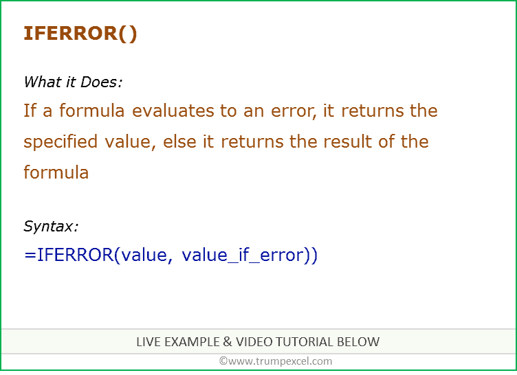752×546 excel iferror function formula examples video from trumpexcel.com

700×400 excel iferror function exceljet from exceljet.net

876×717 iferror function excel remove excel error excel unlocked from excelunlocked.com

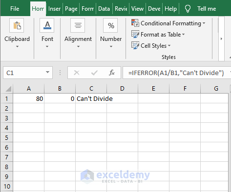473×394 iferror function excel examples exceldemy from www.exceldemy.com

562×479 iferror function excel from www.exceltip.com

1170×1200 iferror professor excel professor excel from professor-excel.com

1200×674 remove errors excel iferror function turbofuture from turbofuture.com

How To Use The Iferror Function To Handle Errors In Excel was posted in August 22, 2025 at 11:36 am. If you wanna have it as yours, please click the Pictures and you will go to click right mouse then Save Image As and Click Save and download the How To Use The Iferror Function To Handle Errors In Excel Picture.. Don’t forget to share this picture with others via Facebook, Twitter, Pinterest or other social medias! we do hope you'll get inspired by ExcelKayra... Thanks again! If you have any DMCA issues on this post, please contact us!