How To Use The Match Function In Excel For Lookups
How To Use The Match Function In Excel For Lookups - There are a lot of affordable templates out there, but it can be easy to feel like a lot of the best cost a amount of money, require best special design template. Making the best template format choice is way to your template success. And if at this time you are looking for information and ideas regarding the How To Use The Match Function In Excel For Lookups then, you are in the perfect place. Get this How To Use The Match Function In Excel For Lookups for free here. We hope this post How To Use The Match Function In Excel For Lookups inspired you and help you what you are looking for.
“`html
Understanding and Utilizing the MATCH Function in Excel for Lookups
The MATCH function in Excel is a powerful, often overlooked tool for performing lookups. While VLOOKUP and INDEX/MATCH are more commonly discussed, understanding the nuances of MATCH alone provides a solid foundation for more complex lookup scenarios. MATCH doesn’t directly return a value like VLOOKUP; instead, it tells you the position of a lookup value within a specified range. This positional information can then be used in conjunction with other functions to extract specific data.
The Syntax of MATCH
The MATCH function has the following syntax:
=MATCH(lookup_value, lookup_array, [match_type])Let’s break down each argument:
- lookup_value: This is the value you’re trying to find within the lookup array. It can be a number, text string, logical value (TRUE/FALSE), or a cell reference.
- lookup_array: This is the range of cells where you want to search for the lookup_value. The lookup array can be a single row or a single column. It’s crucial that the array is contiguous.
- [match_type]: This is an optional argument that controls how Excel searches for the lookup_value. It determines whether the search should be exact, approximate (less than or equal to), or approximate (greater than or equal to). This argument significantly affects the behavior of the function. There are three possible values for match_type:
- 1 (or omitted): Finds the largest value that is less than or equal to lookup_value. Important: The values in the lookup_array must be sorted in ascending order for this option to work correctly. If they aren’t sorted, the result will be unpredictable. This is useful for finding a value within a range, for example, determining which tax bracket a certain income falls into.
- 0: Finds the first value that is exactly equal to lookup_value. The order of values in the lookup_array doesn’t matter. This is the most commonly used option and is essential for exact matches.
- -1: Finds the smallest value that is greater than or equal to lookup_value. Important: The values in the lookup_array must be sorted in descending order for this option to work correctly. If they aren’t sorted, the result will be unpredictable. This is less frequently used but can be useful in specific scenarios.
Illustrative Examples
Let’s explore some practical examples to understand how the MATCH function works in different scenarios.
Example 1: Exact Match (match_type = 0)
Suppose you have a list of employee IDs in cells A1:A10, and you want to find the position of employee ID “1005” within that list. The list is as follows:
A1: 1001 A2: 1003 A3: 1005 A4: 1002 A5: 1008 A6: 1007 A7: 1004 A8: 1006 A9: 1009 A10: 1010
The formula would be:
=MATCH(1005, A1:A10, 0)The result will be 3 because “1005” is the third value in the range A1:A10.
If you wanted to use a cell reference instead of hardcoding the employee ID, and the employee ID was in cell D1, the formula would be:
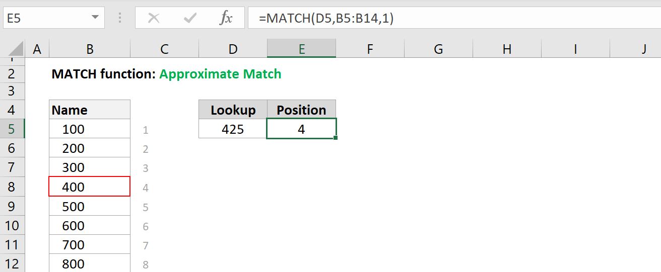
=MATCH(D1, A1:A10, 0)Example 2: Approximate Match (match_type = 1) – Ascending Order
Assume you have a table of sales tiers and corresponding commission rates. You want to determine which commission tier a salesperson belongs to based on their sales amount. The sales tiers are in ascending order:
A1: 0 A2: 1000 A3: 5000 A4: 10000 A5: 20000
And the corresponding commission rates are (for illustration, not used in the MATCH function directly):
B1: 0% B2: 2% B3: 5% B4: 8% B5: 10%
If a salesperson had sales of 7500 (stored in cell C1), the formula to find the appropriate tier would be:
=MATCH(C1, A1:A5, 1)The result will be 3. This is because 7500 is greater than 5000 (A3) but less than 10000 (A4). MATCH returns the position of the largest value in A1:A5 that is less than or equal to 7500, which is 5000 (A3). You can then use this result (3) to find the corresponding commission rate using INDEX, for example: `=INDEX(B1:B5, MATCH(C1, A1:A5, 1))` which would return 5%.
Important Note: If C1 contained a value of -100, the MATCH function would return #N/A because there is no value in A1:A5 less than or equal to -100.
Example 3: Approximate Match (match_type = -1) – Descending Order
Consider a scenario where you have a discount schedule based on order quantity, where discounts decrease as quantity increases. The quantities are listed in descending order:
A1: 100 A2: 50 A3: 20 A4: 10 A5: 0
And the corresponding discount percentages are:
B1: 20% B2: 15% B3: 10% B4: 5% B5: 0%
If an order has a quantity of 35 (in cell C1), the formula to find the applicable discount tier would be:
=MATCH(C1, A1:A5, -1)The result will be 2. This is because 35 is less than 50 (A2) but greater than 20 (A3). MATCH returns the position of the smallest value in A1:A5 that is greater than or equal to 35, which is 50 (A2). You can then use this result (2) to find the corresponding discount using INDEX, such as: `=INDEX(B1:B5, MATCH(C1, A1:A5, -1))` which would return 15%.
Crucial Reminder: For match_type -1 to work correctly, the data in the lookup_array MUST be sorted in descending order.
Common Errors and Troubleshooting
- #N/A Error: This is the most common error encountered with the MATCH function. It indicates that Excel could not find a match for the lookup_value within the lookup_array, according to the specified match_type.
- Exact Match (match_type = 0): Double-check that the lookup_value exists exactly as it appears in the lookup_array. Case sensitivity can be an issue with text values, as well as leading or trailing spaces.
- Approximate Match (match_type = 1 or -1): Ensure that the lookup_array is sorted correctly (ascending for 1, descending for -1). Also, make sure that there is a value within the lookup_array that satisfies the “less than or equal to” (for 1) or “greater than or equal to” (for -1) criteria. For instance, with match_type 1, if the lookup_value is smaller than all values in the lookup_array, you will get #N/A.
- Incorrect Results with Approximate Match: This usually happens when the lookup_array is not sorted correctly when using match_type 1 or -1. Excel relies on the sorted order to perform the approximate match.
- Using MATCH with Non-Contiguous Ranges: The lookup_array in MATCH must be a single continuous range (either a row or a column). You cannot use a non-contiguous range like `(A1:A5, C1:C5)`.
Combining MATCH with INDEX and other Functions
The true power of MATCH lies in its ability to be combined with other Excel functions, particularly INDEX. The INDEX function returns the value at a specific position within a range. By using MATCH to determine the position, and then passing that position to INDEX, you create a dynamic lookup solution.
As seen in the examples above, you can use `INDEX(return_array, MATCH(lookup_value, lookup_array, match_type))` to perform a lookup. This is a flexible alternative to VLOOKUP or HLOOKUP and overcomes some of their limitations, such as the requirement for the lookup column to be the first column in the range.
MATCH can also be combined with functions like OFFSET, INDIRECT, and others to create even more sophisticated and dynamic formulas.
Conclusion
The MATCH function is a fundamental building block for performing lookups in Excel. While it doesn’t directly return values like VLOOKUP, its ability to determine the position of a value within a range makes it incredibly versatile when combined with other functions, especially INDEX. By mastering the nuances of the MATCH function, including the crucial role of the match_type argument and understanding potential error conditions, you can significantly enhance your data analysis and reporting capabilities in Excel.
“`
 1312×541 excel match function excelfind from excelfind.com
  1209×890 match function excel excel glossary perfectxl from www.perfectxl.com
  768×336 excel lookup function excelfind from excelfind.com
  864×598 search matching data match function excel from gyankosh.net
 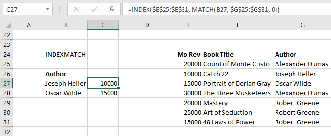 680×281 excel guide lookups matching cells excel shortcut from www.excelshortcut.com
  800×600 lookup function excel steps pictures from www.wikihow.com
 /lookup-function-example-e52c32a8ff5e41b49af6cf2e5ff34f38.png) 1127×752 lookup function excel from www.lifewire.com
1127×752 lookup function excel from www.lifewire.com  300×172 lookup function excel examples lookup function from www.educba.com
 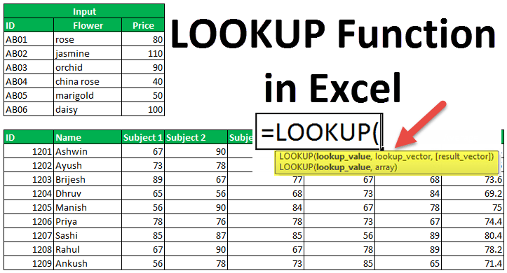 723×390 lookup function excel formula examples from www.wallstreetmojo.com
  474×227 find data excel match function efinancialmodels from www.efinancialmodels.com
  624×395 lookup formula excel index match teachexcelcom from www.teachexcel.com
  922×576 perform approximate match fuzzy lookups excel excel university from www.excel-university.com
  609×369 vlookup match dynamic duo excel campus from www.excelcampus.com
 How To Use The Match Function In Excel For Lookups was posted in December 23, 2025 at 1:46 pm. If you wanna have it as yours, please click the Pictures and you will go to click right mouse then Save Image As and Click Save and download the How To Use The Match Function In Excel For Lookups Picture.. Don’t forget to share this picture with others via Facebook, Twitter, Pinterest or other social medias! we do hope you'll get inspired by ExcelKayra... Thanks again! If you have any DMCA issues on this post, please contact us!