How To Use Vlookup To Find Approximate Match In Excel
How To Use Vlookup To Find Approximate Match In Excel - There are a lot of affordable templates out there, but it can be easy to feel like a lot of the best cost a amount of money, require best special design template. Making the best template format choice is way to your template success. And if at this time you are looking for information and ideas regarding the How To Use Vlookup To Find Approximate Match In Excel then, you are in the perfect place. Get this How To Use Vlookup To Find Approximate Match In Excel for free here. We hope this post How To Use Vlookup To Find Approximate Match In Excel inspired you and help you what you are looking for.
“`html
Finding Approximate Matches with VLOOKUP in Excel
VLOOKUP is a powerful function in Excel used to search for a value in the first column of a table array and return a value in the same row from a specified column. While often used for exact matches, VLOOKUP can also be configured to find approximate matches, which is incredibly useful when you need to find a value that falls within a range or category.
Understanding the VLOOKUP Function
Before delving into approximate matches, let’s briefly recap the VLOOKUP function’s syntax:
=VLOOKUP(lookup_value, table_array, col_index_num, [range_lookup])- lookup_value: The value you want to search for.
- table_array: The range of cells that contains the data you want to search in. The lookup_value is searched in the first column of this range.
- col_index_num: The column number within the table_array from which to return the matching value. The first column is 1, the second is 2, and so on.
- range_lookup: This is the crucial argument for determining whether VLOOKUP performs an exact or approximate match. It’s an optional argument, but specifying it is highly recommended for clarity.
- TRUE (or omitted): Performs an approximate match. The first column of the table_array must be sorted in ascending order. VLOOKUP will return the largest value that is less than or equal to the lookup_value. This is the focus of this article.
- FALSE: Performs an exact match. VLOOKUP will return the value in the same row as the first exact match found for the lookup_value. If an exact match is not found, VLOOKUP returns the #N/A error.
Using VLOOKUP for Approximate Matches
When you set the range_lookup argument to TRUE (or omit it, which defaults to TRUE), VLOOKUP performs an approximate match. This is where things get interesting. Here’s how it works:
- Sorting the Lookup Column: The first column of your
table_arraymust be sorted in ascending order (from smallest to largest) for approximate matching to work correctly. If the data is not sorted, VLOOKUP might return incorrect results or an #N/A error. - Finding the Closest Match: VLOOKUP searches down the first column of the
table_arrayuntil it finds a value that is larger than thelookup_value. It then returns the value from thecol_index_numin the previous row. - Handling Values Smaller Than the Smallest: If the
lookup_valueis smaller than the smallest value in the first column of thetable_array, VLOOKUP will return an #N/A error.
Example: Grade Calculation
Let’s say you have a table that assigns letter grades based on numerical scores:
| Score | Grade |
|---|---|
| 0 | F |
| 60 | D |
| 70 | C |
| 80 | B |
| 90 | A |
This table (let’s assume it’s in the range A1:B6 in your Excel sheet, with headers in row 1) defines the minimum score required for each grade. To use VLOOKUP to determine the grade for a score of 75, you’d use the following formula:
=VLOOKUP(75, A2:B6, 2, TRUE)Here’s how VLOOKUP works in this example:
- lookup_value: 75
- table_array: A2:B6 (The table excluding the header row)
- col_index_num: 2 (We want to retrieve the grade, which is in the second column)
- range_lookup: TRUE (We want an approximate match)
VLOOKUP searches down column A (scores):
- 0 is less than 75.
- 60 is less than 75.
- 70 is less than 75.
- 80 is greater than 75.
Since 80 is greater than 75, VLOOKUP goes back to the previous row (the row containing 70) and returns the value from the second column of that row, which is “C”. Therefore, the formula will return “C”.
Practical Applications of Approximate Match VLOOKUP
Approximate match VLOOKUP is useful in many scenarios, including:
- Tax Brackets: Calculating income tax based on income ranges.
- Commission Rates: Determining commission rates based on sales volume.
- Shipping Costs: Calculating shipping costs based on weight or distance.
- Price Discounts: Applying discounts based on purchase quantity.
- Lookup Tables for Data Categories: Assigning categories to data points based on numeric thresholds.
Important Considerations and Potential Issues
While powerful, using VLOOKUP with approximate matches requires careful attention to detail to avoid errors:
- Sorting is Crucial: The most common mistake is forgetting to sort the first column of the
table_arrayin ascending order. Double-check this before using the formula. Data -> Sort is your friend. - Handling Values Outside the Range: Be aware of what happens when the
lookup_valueis less than the smallest value in the lookup column. VLOOKUP will return an #N/A error. You may need to use IFERROR to handle these cases gracefully. For instance:=IFERROR(VLOOKUP(value, table, column, TRUE), "Value too low") - Gaps in the Data: Ensure there are no unintended gaps in your data. For example, in the grade calculation example, if you skipped the range 60-69, any score in that range would return “F” instead of “D”.
- Alternatives: While VLOOKUP is widely used, other functions like INDEX/MATCH (often paired together) and XLOOKUP offer more flexibility and can sometimes be more efficient. XLOOKUP directly handles missing values and sorting issues, making it a more robust choice if you have Excel 365 or later.
- Error Handling: Use
IFERRORfunction to gracefully handle cases where VLOOKUP returns an error, especially when thelookup_valueis outside the range of thetable_array.
Example: Using IFERROR for Error Handling
Continuing with the grade example, if a score is less than 0 (e.g., -5), VLOOKUP will return an #N/A error. To display a more user-friendly message, you can wrap the VLOOKUP formula with IFERROR:
=IFERROR(VLOOKUP(A10, A2:B6, 2, TRUE), "Invalid Score")In this example, if VLOOKUP returns an error (because the value in cell A10 is less than 0), the formula will display “Invalid Score” instead of #N/A.
Conclusion
VLOOKUP with approximate matches is a valuable tool for categorizing data and performing lookups based on ranges. By understanding how it works and paying attention to the crucial details like sorting and error handling, you can effectively leverage its power in your Excel spreadsheets.
“`
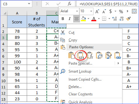 452×338 vlookup approximate match excelnotes from excelnotes.com
  720×232 vlookup exact match approximate match goskills from www.goskills.com
  1024×409 vlookup approximate match myexcelonline from www.myexcelonline.com
  1280×720 excel tutorial troubleshoot vlookup approximate match from exceljet.net
  474×234 vlookup exact approximate match excel from www.extendoffice.com
  1280×720 vlookup approximate match microsoft excel basic advanced from www.goskills.com
  300×140 exact approximate matching vlookup excel from ms-office.wonderhowto.com
 How To Use Vlookup To Find Approximate Match In Excel was posted in January 29, 2026 at 9:47 pm. If you wanna have it as yours, please click the Pictures and you will go to click right mouse then Save Image As and Click Save and download the How To Use Vlookup To Find Approximate Match In Excel Picture.. Don’t forget to share this picture with others via Facebook, Twitter, Pinterest or other social medias! we do hope you'll get inspired by ExcelKayra... Thanks again! If you have any DMCA issues on this post, please contact us!