How To Use Vlookup To Match Partial Text In Excel
How To Use Vlookup To Match Partial Text In Excel - There are a lot of affordable templates out there, but it can be easy to feel like a lot of the best cost a amount of money, require best special design template. Making the best template format choice is way to your template success. And if at this time you are looking for information and ideas regarding the How To Use Vlookup To Match Partial Text In Excel then, you are in the perfect place. Get this How To Use Vlookup To Match Partial Text In Excel for free here. We hope this post How To Use Vlookup To Match Partial Text In Excel inspired you and help you what you are looking for.
“`html
Using VLOOKUP for Partial Text Matching in Excel
The VLOOKUP function in Excel is a powerful tool for searching for a specific value in the first column of a range and then returning a corresponding value from another column in the same row. While traditionally used for exact matches, VLOOKUP can also be adapted to perform partial text matching, allowing you to find values that contain a specific string, even if it’s not an exact match. This capability significantly extends VLOOKUP’s utility, particularly when dealing with messy or inconsistent data.
Understanding the Basics of VLOOKUP
Before diving into partial text matching, let’s quickly review the syntax and purpose of VLOOKUP:
=VLOOKUP(lookup_value, table_array, col_index_num, [range_lookup])- lookup_value: The value you want to search for in the first column of the table array.
- table_array: The range of cells that contains the data you want to search. The first column of this range is where VLOOKUP will look for the `lookup_value`.
- col_index_num: The column number within the `table_array` that contains the value you want to return. The first column is 1, the second is 2, and so on.
- [range_lookup]: An optional argument that specifies whether you want an exact or approximate match.
- TRUE (or omitted): Performs an approximate match. The first column of the `table_array` must be sorted in ascending order. VLOOKUP will return the largest value less than or equal to the `lookup_value`. This is not suitable for partial text matching.
- FALSE: Performs an exact match. VLOOKUP will return the first value that exactly matches the `lookup_value`. If no exact match is found, it will return #N/A.
For partial text matching, we will leverage the `FALSE` argument for exact matching, combined with wildcard characters to broaden the search criteria.
Employing Wildcards for Partial Text Matching
The key to partial text matching with VLOOKUP lies in the use of wildcard characters. Excel supports two primary wildcards:
- Asterisk (*): Represents zero or more characters. For example, `”*apple*”` would match “apple”, “red apple”, “apple pie”, and “pineapple”.
- Question Mark (?): Represents a single character. For example, `”h?t”` would match “hat”, “hot”, and “hit”.
We primarily use the asterisk (*) for partial text matching because it’s more versatile. By incorporating the asterisk into the `lookup_value`, we can tell VLOOKUP to search for cells that *contain* the specified text, rather than requiring an exact match.
Examples of Partial Text Matching with VLOOKUP
Let’s illustrate with some practical examples.
Example 1: Matching Product Names Containing a Specific Keyword
Suppose you have a list of product names in column A (A1:A10) and corresponding prices in column B (B1:B10). You want to find the price of any product that contains the word “apple”.
Here’s the formula you would use:
=VLOOKUP("*"&"apple"&"*", A1:B10, 2, FALSE)Explanation:
- `”*”&”apple”&”*”`: This concatenates an asterisk before and after the word “apple”, creating the lookup value `”*apple*”`. This tells VLOOKUP to find any cell in column A that contains the word “apple”.
- `A1:B10`: This is the table array where VLOOKUP will search.
- `2`: This specifies that we want to return the value from the second column (column B), which contains the prices.
- `FALSE`: This ensures that we’re looking for an exact match of the wildcard-modified lookup value.
If any of the product names in column A contain “apple”, VLOOKUP will return the corresponding price from column B. If no product names contain “apple”, it will return #N/A.
Example 2: Matching Customer Names Starting with a Specific Letter
Assume you have a list of customer names in column C (C1:C20) and their order IDs in column D (D1:D20). You want to find the order ID for any customer whose name starts with the letter “J”.
The formula would be:
=VLOOKUP("J*", C1:D20, 2, FALSE)Explanation:
- `”J*”`: This creates the lookup value “J*”, meaning “J” followed by any number of characters.
- `C1:D20`: The table array containing the customer names and order IDs.
- `2`: The column index number for the order ID (column D).
- `FALSE`: Exact match (of the wildcard-modified lookup value).
Example 3: Using a Cell Reference for the Partial Text
Instead of hardcoding the partial text in the formula, you can use a cell reference. This makes the formula more flexible. Suppose cell F1 contains the text you want to search for (e.g., “banana”). Your product names and prices are still in columns A and B (A1:B10) respectively.
The formula becomes:
=VLOOKUP("*"&F1&"*", A1:B10, 2, FALSE)Now, you can change the value in cell F1, and the VLOOKUP result will update accordingly. This is particularly useful for creating dynamic search tools.
Important Considerations and Limitations
- Case Sensitivity: VLOOKUP is generally not case-sensitive. So, searching for “*apple*” will match both “apple” and “Apple”. If you need case-sensitive matching, you’ll need to use more complex formulas involving functions like `FIND` or `SEARCH` along with `IF` statements.
- Multiple Matches: VLOOKUP only returns the *first* match it finds. If multiple rows contain the partial text you’re searching for, VLOOKUP will only return the value from the first matching row. To retrieve all matches, you’ll need to use more advanced techniques, such as array formulas or VBA.
- Performance: Using wildcards, especially with large datasets, can slow down VLOOKUP’s performance. The more complex your data, the longer it will take to search. Consider optimizing your data or exploring alternative methods if performance becomes an issue.
- Error Handling: If VLOOKUP doesn’t find any matches, it returns the #N/A error. You can use the `IFERROR` function to handle this error and display a more user-friendly message. For example:
=IFERROR(VLOOKUP("*"&"apple"&"*", A1:B10, 2, FALSE), "Product not found") - Data Type Consistency: Ensure that the data type of your `lookup_value` is consistent with the data type in the first column of your `table_array`. If you’re searching for a number, make sure the first column of your table array contains numbers, not text.
- Using INDEX and MATCH for More Flexibility: While VLOOKUP is useful, the `INDEX` and `MATCH` functions offer more flexibility. They allow you to search in any column and return values from any other column, without the limitations imposed by VLOOKUP’s requirement that the lookup value be in the first column. For complex scenarios, `INDEX` and `MATCH` are often a better choice.
- Alternatives to VLOOKUP: Functions like `XLOOKUP` (available in newer versions of Excel) offer enhanced features, including built-in support for partial matching and the ability to search from bottom to top. `FILTER` is another very powerful function that can be used in place of many VLOOKUP scenarios, particularly when you want to return multiple matches.
Conclusion
Partial text matching with VLOOKUP, using wildcards, is a valuable technique for data analysis and manipulation in Excel. By understanding how to use the asterisk (*) and question mark (?) wildcards effectively, you can significantly expand the capabilities of VLOOKUP and handle a wider range of data scenarios. Remember to consider the limitations and potential performance implications, and explore alternative functions like `INDEX/MATCH`, `XLOOKUP`, and `FILTER` when appropriate. Always handle potential errors gracefully using `IFERROR` for a more robust and user-friendly solution.
“`
 650×421 vlookup partial match excel teachexcelcom from www.teachexcel.com
  566×369 partial match lookup numbers excel teachexcelcom from www.teachexcel.com
  828×281 vlookup partial match excel google sheets automate excel from www.automateexcel.com
  673×503 partial vlookup match part excel from online-excel-training.auditexcel.co.za
 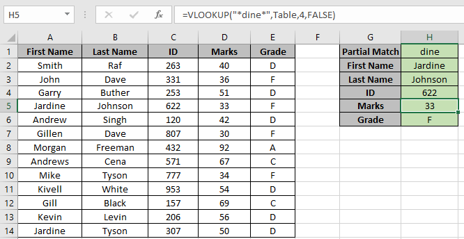 666×344 partial match vlookup function from www.exceltip.com
 How To Use Vlookup To Match Partial Text In Excel was posted in March 6, 2026 at 5:05 am. If you wanna have it as yours, please click the Pictures and you will go to click right mouse then Save Image As and Click Save and download the How To Use Vlookup To Match Partial Text In Excel Picture.. Don’t forget to share this picture with others via Facebook, Twitter, Pinterest or other social medias! we do hope you'll get inspired by ExcelKayra... Thanks again! If you have any DMCA issues on this post, please contact us!