Vlookup Approximate Match Tutorial Excel For Beginners
Vlookup Approximate Match Tutorial Excel For Beginners - There are a lot of affordable templates out there, but it can be easy to feel like a lot of the best cost a amount of money, require best special design template. Making the best template format choice is way to your template success. And if at this time you are looking for information and ideas regarding the Vlookup Approximate Match Tutorial Excel For Beginners then, you are in the perfect place. Get this Vlookup Approximate Match Tutorial Excel For Beginners for free here. We hope this post Vlookup Approximate Match Tutorial Excel For Beginners inspired you and help you what you are looking for.
VLOOKUP Approximate Match Tutorial for Excel Beginners
VLOOKUP is one of Excel’s most powerful and frequently used functions. While many tutorials focus on exact matches, the approximate match feature opens up a whole new range of possibilities, especially when dealing with categories, grades, or tiered pricing. This guide will walk you through how to use VLOOKUP with approximate match, explaining the concept, syntax, and providing practical examples suitable for beginners.
Understanding VLOOKUP
Before diving into approximate match, let’s briefly recap what VLOOKUP does. VLOOKUP, short for “Vertical Lookup,” searches for a value in the first column of a table and then returns a corresponding value from a column you specify. Think of it like looking up a word in a dictionary; you find the word (the lookup value) and then read its definition (the returned value).
The general syntax for VLOOKUP is:
=VLOOKUP(lookup_value, table_array, col_index_num, [range_lookup])
Where:
- lookup_value: The value you want to find in the first column of the table.
- table_array: The range of cells containing the table where you want to look up the value. Remember to use absolute references ($A$1:$C$10) if you plan to copy the formula.
- col_index_num: The column number in the table_array from which you want to return a value. The first column is 1, the second is 2, and so on.
- [range_lookup]: This is the crucial argument for determining whether you want an exact or approximate match. It’s optional, but understanding it is key to using VLOOKUP effectively.
When range_lookup is:
- TRUE or omitted: VLOOKUP will find an approximate match. The first column of the table array MUST be sorted in ascending order. VLOOKUP will return the largest value in the first column that is less than or equal to the lookup_value.
- FALSE: VLOOKUP will find an exact match. If an exact match is not found, VLOOKUP will return the #N/A error.
The Power of Approximate Match
The real magic of VLOOKUP often lies in its ability to find *approximate* matches. This is incredibly useful in scenarios where you don’t need (or even want) a perfectly identical value. Think about scenarios like:
- Grading systems: A score of 85 earns a “B,” but you don’t need a cell containing exactly “85” to assign that grade. Any score between 80 and 89 should result in a “B.”
- Commission tiers: Sales above $10,000 earn a 5% commission, but you’re unlikely to have a sales figure of precisely $10,000.
- Shipping costs: Weight ranges determine shipping fees (e.g., 0-1 lb costs $5, 1-5 lbs costs $10).
In these cases, using VLOOKUP with an approximate match simplifies your calculations and eliminates the need for complex IF statements.
Example: Grading System
Let’s create a simple grading system using VLOOKUP approximate match.
- Set up your grading table:
In a new Excel sheet, create a table with the minimum score for each grade and the corresponding grade letter. It’s crucial that the minimum scores are sorted in ascending order.
For example:
Minimum Score Grade 0 F 60 D 70 C 80 B 90 A Let’s assume this table is located in cells
A1:B6(including headers). - Enter student scores:
In another column (e.g., column D), enter the scores you want to grade.
For example:
Student Score Alice 85 Bob 72 Charlie 95 David 55 Let’s assume these scores are in cells
E2:E5. - Apply the VLOOKUP formula:
In the column next to the scores (e.g., column F), enter the VLOOKUP formula to calculate the grade. In cell
F2, enter:=VLOOKUP(E2, $A$2:$B$6, 2, TRUE)Let’s break this down:
E2: This is the lookup value – the student’s score we want to find a grade for.$A$2:$B$6: This is the table array containing the minimum scores and grades. The dollar signs create absolute references, ensuring the table array doesn’t change when you copy the formula down. We start at A2 to exclude the headers.2: This is the column index number. We want to retrieve the grade from the *second* column of the table array (the “Grade” column).TRUE: This tells VLOOKUP to perform an *approximate* match. Since it’s TRUE (or omitted), Excel expects the first column of our table to be sorted in ascending order, and it will return the largest value in the first column that’s less than or equal to the score.
- Copy the formula down:
Click and drag the bottom-right corner of cell
F2down toF5to apply the formula to all students. Excel will automatically adjust theE2reference toE3,E4, andE5for each student.
The results should be:
| Student | Score | Grade |
|---|---|---|
| Alice | 85 | B |
| Bob | 72 | C |
| Charlie | 95 | A |
| David | 55 | F |
Notice how VLOOKUP correctly assigns the grades based on the score ranges. For example, Alice’s score of 85 falls between the minimum scores for a “B” (80) and an “A” (90), so VLOOKUP returns “B.” David’s score is below 60, so VLOOKUP returns “F”.
Important Considerations for Approximate Match
- Sorted First Column: The *most crucial* requirement for approximate match is that the first column of your
table_array**must be sorted in ascending order.** If it’s not, VLOOKUP might return incorrect results or an error. - Lowest Value: Include the lowest possible value in your table (often zero) to ensure that any values below your first threshold are handled correctly. In the grading example, without ‘0’ assigned to F, David would return an error since no minimum bound was set.
- Headers: When defining your
table_array, consider whether you want to include the headers. In the examples, we exclude them, and started with the actual data in the table. - Error Handling: While VLOOKUP with approximate match is powerful, consider adding error handling (using
IFERROR) to gracefully handle unexpected input values.
Conclusion
VLOOKUP with approximate match is a valuable tool for any Excel user. By understanding how it works and remembering the key requirement of a sorted first column, you can simplify calculations, automate grading systems, and perform other complex lookups with ease. Practice with different scenarios and explore the IFERROR function for more robust solutions.
 768×334 vlookup approximate match myexcelonline from www.myexcelonline.com
  1280×720 excel tutorial troubleshoot vlookup approximate match from exceljet.net
 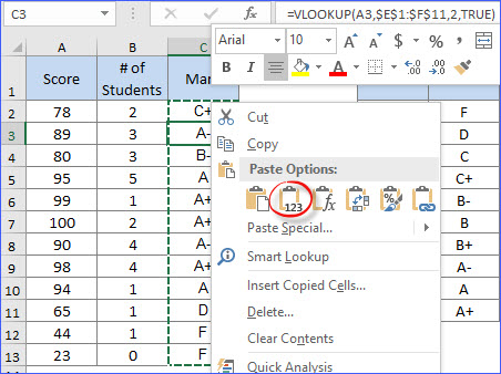 452×338 vlookup approximate match excelnotes from excelnotes.com
  1187×477 vlookup exact approximate match excel from www.extendoffice.com
  1280×720 vlookup approximate match microsoft excel basic advanced from www.goskills.com
 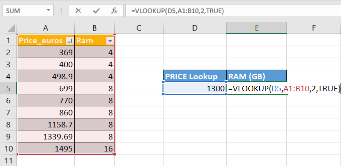 680×331 mastering vlookup excel step step guide from www.simplilearn.com
  405×297 excel vlookup tutorial beginners formula examples from ablebits.com
  1280×600 exact approximate matching vlookup excel from ms-office.wonderhowto.com
 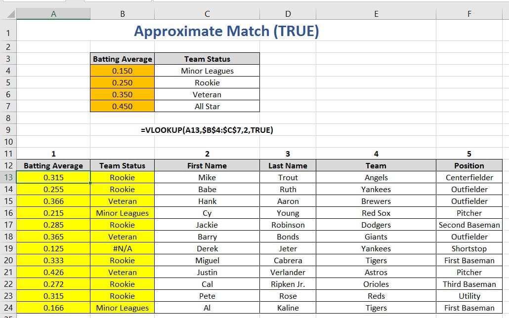 1030×644 vlookup function excel excelbuddycom from excelbuddy.com
 Vlookup Approximate Match Tutorial Excel For Beginners was posted in March 4, 2026 at 2:17 am. If you wanna have it as yours, please click the Pictures and you will go to click right mouse then Save Image As and Click Save and download the Vlookup Approximate Match Tutorial Excel For Beginners Picture.. Don’t forget to share this picture with others via Facebook, Twitter, Pinterest or other social medias! we do hope you'll get inspired by ExcelKayra... Thanks again! If you have any DMCA issues on this post, please contact us!