How To Use Conditional Formatting For Due Dates In Excel
How To Use Conditional Formatting For Due Dates In Excel - There are a lot of affordable templates out there, but it can be easy to feel like a lot of the best cost a amount of money, require best special design template. Making the best template format choice is way to your template success. And if at this time you are looking for information and ideas regarding the How To Use Conditional Formatting For Due Dates In Excel then, you are in the perfect place. Get this How To Use Conditional Formatting For Due Dates In Excel for free here. We hope this post How To Use Conditional Formatting For Due Dates In Excel inspired you and help you what you are looking for.
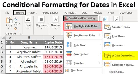
Conditional Formatting for Due Dates in Excel Conditional formatting in Excel is a powerful tool that allows you to visually highlight cells based on specific criteria. When managing tasks and deadlines, using conditional formatting for due dates can dramatically improve your organization and efficiency. This guide will walk you through various scenarios and techniques to effectively use conditional formatting for due dates in Excel. **Understanding the Basics** Before diving into specific examples, let’s establish the fundamentals of conditional formatting. The core concept involves defining rules that Excel evaluates for each cell within a selected range. If a cell meets the conditions defined in a rule, the specified formatting is applied, making it easy to spot critical information at a glance. **Accessing Conditional Formatting** To access conditional formatting options, select the range of cells you want to apply the formatting to. Then, navigate to the “Home” tab on the Excel ribbon and click on “Conditional Formatting” in the “Styles” group. This will open a dropdown menu with various options, including preset rules and the option to create your own custom rules. **Scenario 1: Highlighting Overdue Dates** The most common use case is to highlight dates that have already passed. This allows you to immediately identify tasks that are behind schedule. 1. **Select the Range:** Select the column containing the due dates you want to monitor. For instance, if your due dates are in column ‘C’, select the range ‘C2:C100’ (adjust the range according to your data). 2. **Create a New Rule:** Go to “Home” -> “Conditional Formatting” -> “New Rule…”. 3. **Choose a Rule Type:** In the “New Formatting Rule” dialog box, select “Use a formula to determine which cells to format”. 4. **Enter the Formula:** In the formula box, enter the following formula: `=C2 “Conditional Formatting” -> “New Rule…”. 3. **Choose a Rule Type:** Select “Use a formula to determine which cells to format”. 4. **Enter the Formula:** In the formula box, enter the following formula: `=AND(C2>=TODAY(),C2<=TODAY()+7)` * `C2` refers to the first cell in your selected range. * `TODAY()` returns the current date. * `TODAY()+7` calculates the date seven days from today. * `AND()` is a logical function that requires both conditions to be true for the formatting to be applied. This formula checks if the date in C2 is greater than or equal to today's date AND less than or equal to today's date plus seven days. 5. **Format the Cells:** Click the "Format..." button and choose a formatting style, such as a yellow fill color. 6. **Apply the Rule:** Click "OK" in both dialog boxes to apply the rule. This rule will highlight dates that are within the next seven days with the chosen format. **Scenario 3: Dynamic Highlighting Based on Status (Completed vs. Incomplete)** You can also combine conditional formatting with other columns, such as a "Status" column, to only highlight due dates if the task is not yet completed. 1. **Assume Status is in Column 'D':** Suppose your "Status" (e.g., "Completed", "In Progress", "Not Started") is in column 'D'. 2. **Select the Range (Due Dates Column):** Select the column containing the due dates (e.g., 'C2:C100'). 3. **Create a New Rule:** Go to "Home" -> “Conditional Formatting” -> “New Rule…”. 4. **Choose a Rule Type:** Select “Use a formula to determine which cells to format”. 5. **Enter the Formula:** To highlight overdue dates only if the status is not “Completed”, use the following formula: `=AND(C2“Completed”)` * `C2` refers to the first date cell. * `D2` refers to the first status cell. * `D2<>“Completed”` checks if the value in cell D2 is not equal to “Completed”. 6. **Format the Cells:** Click the “Format…” button and choose a formatting style (e.g., red fill). 7. **Apply the Rule:** Click “OK” in both dialog boxes. This will highlight overdue dates only if the corresponding status is not “Completed.” You can adapt the formula to match your specific status values. **Scenario 4: Using Icons Sets for Visual Cues** Excel’s icon sets provide another way to visually represent due dates. 1. **Select the Range:** Select the range of due dates. 2. **Go to Conditional Formatting:** “Home” -> “Conditional Formatting” -> “Icon Sets”. 3. **Choose an Icon Set:** Select a suitable icon set, such as the “3 Arrows (Colored)” set. 4. **Modify the Rule (Optional):** To customize the icon set thresholds, go to “Home” -> “Conditional Formatting” -> “Manage Rules…”. Select the icon set rule and click “Edit Rule…”. You can then change the icon set and the values used to assign each icon. For example, you could set thresholds so that: * Green Arrow (Pointing Up): Date is in the future (>=TODAY()) * Yellow Arrow (Pointing Sideways): Date is within the next 7 days (>=TODAY() AND <=TODAY()+7) * Red Arrow (Pointing Down): Date is overdue ( “Conditional Formatting” -> “Manage Rules…”. This will open the “Conditional Formatting Rules Manager” dialog box. Here, you can: * **View Rules:** See all conditional formatting rules applied to the current selection or the entire worksheet. * **Edit Rules:** Modify existing rules, including the formula, formatting style, and range. * **Delete Rules:** Remove unwanted rules. * **Change Rule Order:** Adjust the order in which rules are applied. Rules are applied from top to bottom, and the first rule that matches a cell’s value will be applied. This is important if you have multiple rules that might overlap. **Best Practices** * **Use Clear and Consistent Formatting:** Choose formatting styles that are easily distinguishable and consistently applied. * **Use Relative References:** When using formulas, use relative cell references (e.g., `C2`) so the formula adapts to each cell in the selected range. * **Test Your Rules:** After creating a rule, test it thoroughly with different dates to ensure it works as expected. * **Combine with Other Excel Features:** Leverage other Excel features like filters and sorting to further analyze and manage your due dates. By implementing these conditional formatting techniques, you can effectively manage your due dates in Excel, improving your organization and productivity.
 542×256 due conditional formatting excel tips mrexcel publishing from www.mrexcel.com
 460×223 conditional formatting highlight due excel learn from fiveminutelessons.com
 700×400 excel formula conditional formatting date due exceljet from exceljet.net
653×354 conditional formatting excel examples from www.educba.com
 521×424 highlight rows conditional formatting excel from www.excelcampus.com
 700×400 excel formula conditional formatting gantt chart exceljet from exceljet.net
 540×248 highlight due excel tips mrexcel publishing from www.mrexcel.com
 387×372 excel conditional formatting time formula examples rules from ablebits.com
How To Use Conditional Formatting For Due Dates In Excel was posted in October 30, 2025 at 10:41 am. If you wanna have it as yours, please click the Pictures and you will go to click right mouse then Save Image As and Click Save and download the How To Use Conditional Formatting For Due Dates In Excel Picture.. Don’t forget to share this picture with others via Facebook, Twitter, Pinterest or other social medias! we do hope you'll get inspired by ExcelKayra... Thanks again! If you have any DMCA issues on this post, please contact us!
 542×256 due conditional formatting excel tips mrexcel publishing from www.mrexcel.com
 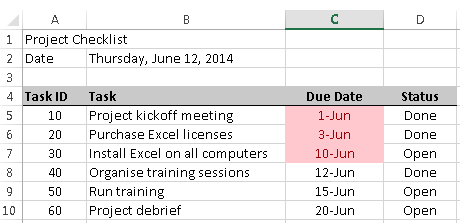 460×223 conditional formatting highlight due excel learn from fiveminutelessons.com
  700×400 excel formula conditional formatting date due exceljet from exceljet.net
  653×354 conditional formatting excel examples from www.educba.com
 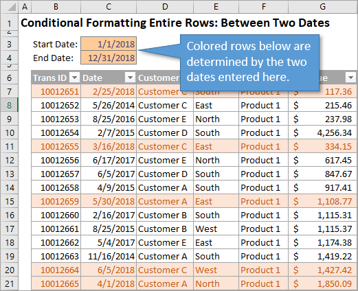 521×424 highlight rows conditional formatting excel from www.excelcampus.com
  700×400 excel formula conditional formatting gantt chart exceljet from exceljet.net
  540×248 highlight due excel tips mrexcel publishing from www.mrexcel.com
  387×372 excel conditional formatting time formula examples rules from ablebits.com